Postgres: B+tree scalar array search and skip scan

PostgreSQL 18 shipped with a bunch of nice features, and since I have been knee-deep into database indexes lately, one feature that piqued my interest is "skip scan" for B+ tree indexes. So I dug deeper into its implementation to understand how it works.

Before proceeding, I should mention that understanding this article requires a decent understanding of B+ trees, so I'd recommend getting familiar with that first if you're not already. For an overview of B+ trees, the wikipedia page is a decent resource, usetheindexluke is a straightfoward resource on indexes generally. This simulator is a good tool for understanding its structure.

Skip scan allows for an efficient index scan:

When the scan key is a non-leading attribute in a multi-column index.
When there are range scan keys on a leading attribute in a multi-column index, e.g., queries with inequality operators: <,>, <=, >=, != , NOT NULL, BETWEEN.

In this article I'll focus on the first (I'll write about the second in a follow-up).

Given a multi-column index (dept_id, emp_id), an index scan WHERE dept_id = ?? will be efficient, but without skip scan, WHERE emp_id = ?? scan will be inefficient.

The image below shows the scan path for a query WHERE dept_id = 42 on a simplified (dept_id, emp_id) B+ tree index.

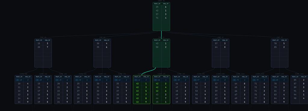
The scan is able to descend directly to the leaf page that contains the matching tuples. This is because the index is sorted first by dept_id.

Now, consider a query WHERE emp_id = 5. The image below shows the scan path to retrieve all matching entries in the same index:

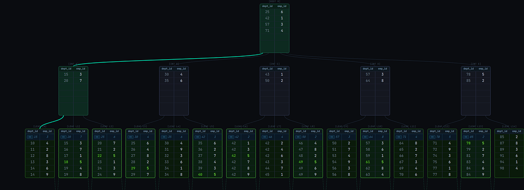
It descends to the leftmost leaf page and then traverses the leaf pages linearly from leftmost to rightmost. Inefficient!

One obvious solution will be to create a new index with emp_id as the leading column. But more indexes affect writes. With skip scan, the same index could be used efficiently for the query.

To understand skip scan, first we need to understand how index scans for scalar array operators work, specifically queries with the IN operator with a scalar list.

How scalar array searches work

Given a query with WHERE dept_id IN (10, 20, 30, 40, 50, 70, 90) AND emp_id = 5, multiple index scans, 1 per combination of each element in the dept_id IN array and emp_id will be executed. The scan will typically work as illustrated in Fig. 3 and as described in the steps below:

The first scan key is (10, 5). The B+tree descent leads to the first leaf page that may contain tuples matching the scan key.
Execute a binary search on the leaf page. This returns the first tuple >= the scan key.
If the found tuple is not equal to the scan key (i.e., it's >), it means there are no tuples matching the scan key. We could end the index scan for the current scan key, advance the current dept_id array element to the next element (20) and begin a new index scan with the new scan key (20, 5) (actually that's what would happen prior to Postgres 17). But instead of just advancing to the next array element, it might be possible to advance even further, so the following is done (Postgres >= 17):
1. Binary search the dept_id IN array for the first element >= the tuple's dept_id value.
2. If the binary search returned an element >= the tuple's value, advance the current array element for
  dept_id to that element. In the illustration below, the search returned 50, the new scan key will be (50, 5) (so we were able to skip over 20 , 30, and 40).
3. Else, it means the tuple is greater than all the array elements, so there'll never be a match for any of the elements, so the entire index scan ends.
If the found tuple (from step 2) is equal to the scan key or if after a scan key array advancement (from step 3.2), the tuple is equal to the new scan key, store the tuple in a results buffer. Continue linearly to the next tuples in the page, storing matching tuples in the results buffer. When we encounter a tuple > the scan key, loop back to step 3.1.
If after an array advancement, the current tuple is < the scan key, it means matching tuples might be ahead. We could keep crawling the page linearly until we find matching tuples, but we don't want to waste our time if we won't find any. To avoid that, a "lookahead" optimization is used:
1. Compare the scan key with the page's last tuple.
2. If it's <=, then it means we might find matching tuples on the current page, so continue the linear traversal through tuples on the page until we get to the start of matching ones (then we'll loop back to step 4).
3. If it's >, then it means we won't find matching tuples on this page. We could check if the next page starts with matching tuples. Postgres' B+ tree implementation stores the value of the next page's (i.e., right sibling's) first tuple in a "pivot tuple" in the current page (this tuple is called a HI KEY, labeled HK in the diagrams). This allows us to peek at the next page's starting tuple without visiting the page. So:
4. 1. Compare the scan key with the tuple.
  2. If the scan key is equal, move to the page and loop back to step 4.
  3. If the scan key is greater, there may or may not be matching tuples on that page. Going to the page to continue the scan and not finding matching tuples would be costly, so we won't risk it. So end the current index scan and start a new one (loop back to step 1) with the scan key, so that we go directly to the leaf page that is certain to either yield matching tuples or end the scan.
  4. If the scan key is lower, it means we won't find any more matching tuples for the current scan key, so loop to 3.1 to advance the array scan key. After advancement, the current index scan ends and a new one with the new scan key starts (if the array elements aren't exhausted).
The entire scan ends when the array elements have been exhausted.

How Skip scan works

Skip scan is based on the same array search mechanism.

When the scan key is a non-leading column, a fake array scan key on the leading column is created. A few details about this fake array:

It won't have any defined elements; instead, the current element is determined based on actual tuple values.
The array is advanced by incrementing the value of the current element by 1 (Note: only scalar data types support this currently: integers, char, timestamp, etc.)
The maximum element is the maximum value of the scan key's data type. E.g., 2147483647 if it's a signed integer.

Using the earlier example: Searching for emp_id = 5 on a (dept_id, emp_id) index, the steps are very similar to the scalar array search. The steps are described below and illustrated in Fig. 4:

Descend the tree to the leftmost page leaf page
Set the current element for dept_id to the tuple's value. In the example, the value is 1, so the scan key becomes (1, 5)
If the tuple is > the scan key, it means there are no tuples matching the scan key. Increment the current element for dept_id, so the new scan key becomes (2, 5).
If the tuple is < the scan key (either initially or after incrementing the scan key), it means matching tuples could be ahead, so utilize "lookahead" optimization (exactly the same as step 5 of the scalar array search):
1. Compare the scan key with the page's last tuple.
2. If the scan key is <=, then it means we might find matching tuples on the current page, so continue linearly to the next tuples until we get to the start of matching ones (then we'll jump to step 5).
3. If it's >, then it means we won't find matching tuples on this page.
4. 1. Compare the scan key with the HI KEY (i.e., the first tuple value of the next page) to check if the next page starts with matching tuples:
  2. If the scan key is equal, move to that page and loop back to step 4.
  3. If the scan key is greater, end the current index scan and start a new one with the scan key, so that we go directly to the leaf page that is certain to either yield matching tuples or end the scan.
  4. If the scan key is lower, it means we won't find any more matching tuples for the current scan key, so loop back to step 3 to advance the array scan key. After advancement, the current index scan ends and a new one with the new scan key starts.
If the tuple is equal to the scan key (either initially or after incrementing the scan key), continue linearly to the next tuples in the page, storing matching tuples in the results buffer. As soon as we encounter a tuple > the scan key, loop to step 2 to set the current element for dept_id to the tuple's value.
If we get to the last tuple of the page, loop to 4.3.1 for possible next page advancement (based on HI KEY).
If the current index scan ended (in 4.3.4), a new index scan with the latest scan key starts as follows:
1. The B+tree descent leads to the first leaf page that may contain tuples matching the scan key.
2. Execute a binary search on the leaf page. This returns the first tuple >= the scan key.
3. Continue from step 4.
The entire index scan ends when either incrementing the scan key will result in an integer overflow (unlikely) or we're at the right-most page.

As seen in the GIF, the skip scan isn't really efficient. It executes many index scans and visits most of the leaf pages. A linear scan of the leaf pages from leftmost to rightmost (as illustrated in Fig. 2) could have even been better.

This brings us to a fact:

Skip scan is inefficient and possibly pointless when the leading column has high cardinality.

There are over 100 unique values for dept_id in the index.

Now let's examine skip scan when dept_id has only 3 unique values in Fig. 5

The scan visits only 4 leaf pages to retrieve all matching tuples! That's fast. Without skip scan, it'd have been a linear scan of leaf pages from leftmost to rightmost as in Fig. 2.

Real database examples

Create a table: positions_low_cardinality with the following script:

CREATE TABLE positions_low_cardinality (dept_id integer, emp_id integer);

INSERT INTO
  positions_low_cardinality (dept_id, emp_id)
SELECT
  (random() * 10) :: integer AS dept_id,
  (random() * 1000000) :: integer AS emp_id
FROM
  generate_series(1, 10000000) AS id;

CREATE INDEX idx_positions_low_cardinality_dept_id_emp_id ON positions_low_cardinality (dept_id, emp_id);

The table has 2 columns: dept_id, emp_id and a (dept_id, emp_id) index. We also insert 10 million records with random values for dept_id and emp_id; dept_id has at most 10 unique values.

Running the following query on Postgres 17 (no skip scan) (Note: we need to force an index scan by nudging the planner to not choose a sequential scan by setting enable_seqscan = off):

SET enable_seqscan = off;
EXPLAIN (ANALYZE,BUFFERS) SELECT COUNT(*) FROM positions_low_cardinality WHERE emp_id = 5;

It yields this:

 Aggregate  (cost=171948.41..171948.42 rows=1 width=8) (actual time=1012.288..1012.289 rows=1 loops=1)
   Buffers: shared hit=1 read=24152
   ->  Index Only Scan using idx_positions_low_cardinality_dept_id_emp_id on positions_low_cardinality  (cost=0.43..171948.38 rows=12 width=0) (actual time=120.106..1003.310 rows=10 loops=1)
         Index Cond: (emp_id = 5)
         Heap Fetches: 0
         Buffers: shared hit=1 read=24152
 Planning Time: 1.749 ms
 JIT:
   Functions: 3
   Options: Inlining false, Optimization false, Expressions true, Deforming true
   Timing: Generation 5.641 ms (Deform 0.000 ms), Inlining 0.000 ms, Optimization 1.775 ms, Emission 7.150 ms, Total 14.566 ms
 Execution Time: 1019.134 ms
(12 rows)

The execution time was 1019ms with 24153 pages accessed. This is because the scan traversed the leaf pages linearly from the leftmost to the rightmost pages, as illustrated in Fig. 2.

Now copy the table and index to a v18 database to ensure we have the exact same data. A simple pg_dump v17 | psql v18 copy should suffice.

Running the same query on the v18 database (with skip scan) yields:

 Aggregate  (cost=57.45..57.46 rows=1 width=8) (actual time=0.480..0.482 rows=1.00 loops=1)
   Buffers: shared hit=38
   ->  Index Only Scan using idx_positions_low_cardinality_dept_id_emp_id on positions_low_cardinality  (cost=0.43..57.42 rows=11 width=0) (actual time=0.278..0.457 rows=10.00 loops=1)
         Index Cond: (emp_id = 5)
         Heap Fetches: 0
         Index Searches: 12
         Buffers: shared hit=38
 Planning Time: 0.326 ms
 Execution Time: 0.644 ms

A hell of a difference, isn't it?

The execution time was 0.644ms with only 38 pages accessed. The scan here was similar to Fig. 5. The skip scan was efficient because the leading column dept_id has low cardinality; only 10 unique values.

Now let's test the same query on a table with high cardinality on dept_id.

CREATE TABLE positions_high_cardinality (dept_id integer, emp_id integer);

INSERT INTO
  positions_high_cardinality (dept_id, emp_id)
SELECT
  (random() * 100000) :: integer AS dept_id,
  (random() * 1000000) :: integer AS emp_id
FROM
  generate_series(1, 10000000) AS id;


CREATE INDEX idx_positions_high_cardinality_dept_id_emp_id ON positions_high_cardinality (dept_id, emp_id);

On Postgres 17 (no skip scan):

 Aggregate  (cost=184688.40..184688.41 rows=1 width=8) (actual time=621.260..621.261 rows=1 loops=1)
   Buffers: shared hit=4 read=27325
   ->  Index Only Scan using idx_positions_high_cardinality_dept_id_emp_id on positions_high_cardinality  (cost=0.43..184688.37 rows=11 width=0) (actual time=141.168..615.807 rows=7 loops=1)
         Index Cond: (emp_id = 5)
         Heap Fetches: 0
         Buffers: shared hit=4 read=27325
 Planning Time: 3.073 ms
 JIT:
   Functions: 3
   Options: Inlining false, Optimization false, Expressions true, Deforming true
   Timing: Generation 3.379 ms (Deform 0.000 ms), Inlining 0.000 ms, Optimization 0.644 ms, Emission 4.769 ms, Total 8.793 ms
 Execution Time: 625.741 ms
(12 rows)

On Postgres 18 (with skip scan):

 Aggregate  (cost=184707.22..184707.23 rows=1 width=8) (actual time=550.163..550.164 rows=1.00 loops=1)
   Buffers: shared hit=3 read=27326
   ->  Index Only Scan using idx_positions_high_cardinality_dept_id_emp_id on positions_high_cardinality  (cost=0.43..184707.19 rows=11 width=0) (actual time=139.729..541.799 rows=7.00 loops=1)
         Index Cond: (emp_id = 5)
         Heap Fetches: 0
         Index Searches: 1
         Buffers: shared hit=3 read=27326
 Planning Time: 2.111 ms
 JIT:
   Functions: 3
   Options: Inlining false, Optimization false, Expressions true, Deforming true
   Timing: Generation 3.890 ms (Deform 0.000 ms), Inlining 0.000 ms, Optimization 1.407 ms, Emission 6.919 ms, Total 12.216 ms
 Execution Time: 557.444 ms
(13 rows)

The execution time and pages accessed were similar, inefficient in both databases! This shows the value of skip scan diminishes with higher cardinality on the leading index column.

In a subsequent article, I'll cover how skip scan optimizes queries with range scan keys, e.g., queries with inequality operators: <,>, <=, >=, != , NOT NULL, BETWEEN.